Contributed by: Egor Romanov
Supabase Vector is about to get a lot faster. New Supabase databases will ship with pgvector v0.5.0 which adds a new type of index: Hierarchical Navigable Small World (HNSW).
HNSW is an algorithm for approximate nearest neighbor search, often used in high-dimensional spaces like those found in embeddings.
With this update, you can take advantage of the new HNSW index on your column using the following:
_10-- Add a HNSW index for the inner product distance function_10CREATE INDEX ON documents_10USING hnsw (embedding vector_ip_ops);
How does HNSW work?
Compared to inverted file (IVF) indexes which use clusters to approximate nearest-neighbor search, HNSW uses proximity graphs (graphs connecting nodes based on distance between them). To understand HNSW, we can break it down into 2 parts:
- Hierarchical (H): The algorithm operates over multiple layers
- Navigable Small World (NSW): Each vector is a node within a graph and is connected to several other nodes
Hierarchical
The hierarchical aspect of HNSW builds off of the idea of skip lists.
Skip lists are multi-layer linked lists. The bottom layer is a regular linked list connecting an ordered sequence of elements. Each new layer above removes some elements from the underlying layer (based on a fixed probability), producing a sparser subsequence that “skips” over elements.
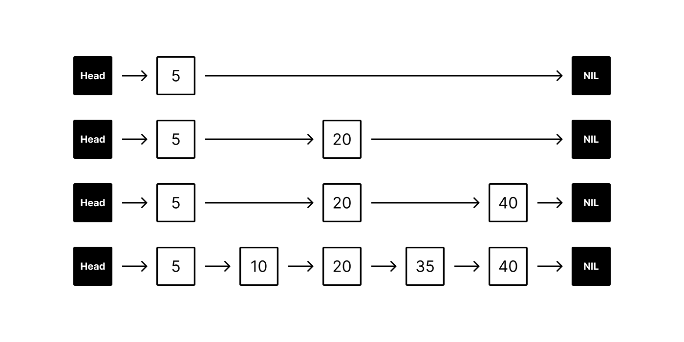
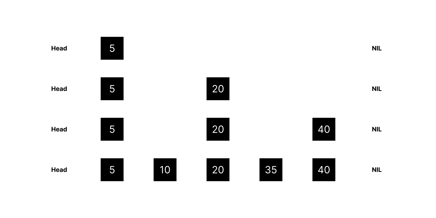
When searching for an element, the algorithm begins at the top layer and traverses its linked list horizontally. If the target element is found, the algorithm stops and returns it. Otherwise if the next element in the list is greater than the target (or NIL), the algorithm drops down to the next layer below. Since each layer below is less sparse than the layer above (with the bottom layer connecting all elements), the target will eventually be found. Skip lists offer O(log n) average complexity for both search and insertion/deletion.
Navigable Small World
A navigable small world (NSW) is a special type of proximity graph that also includes long-range connections between nodes. These long-range connections support the “small world” property of the graph, meaning almost every node can be reached from any other node within a few hops. Without these additional long-range connections, many hops would be required to reach a far-away node.
The “navigable” part of NSW specifically refers to the ability to logarithmically scale the greedy search algorithm on the graph, an algorithm that attempts to make only the locally optimal choice at each hop. Without this property, the graph may still be considered a small world with short paths between far-away nodes, but the greedy algorithm tends to miss them. Greedy search is ideal for NSW because it is quick to navigate and has low computational costs.
Hierarchical + Navigable Small World
HNSW combines these two concepts. From the hierarchical perspective, the bottom layer consists of a NSW made up of short links between nodes. Each layer above “skips” elements and creates longer links between nodes further away from each other.
Just like skip lists, search starts at the top layer and works its way down until it finds the target element. However instead of comparing a scalar value at each layer to determine whether or not to descend to the layer below, a multi-dimensional distance measure (such as Euclidean distance) is used.
HNSW performance: 1536 dimensions
To understand the performance improvements that HNSW offers, we decided to expand upon our previous benchmarks and include results for the HNSW index in addition to IVF and compare the queries per second (QPS) for both.
wikipedia-en-embeddings
In the first test, we used 224,482 vectors by OpenAI (1536 dimensions). You can find our previous benchmark with additional information on how vector dimensions may affect performance in pgvector: Fewer dimensions are better.
In this test, we used a Supabase project with a large compute add-on (2-core CPU and 8GB RAM) and built the HNSW index with the following parameters:
m: 32ef_construction: 64
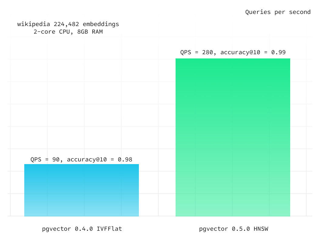
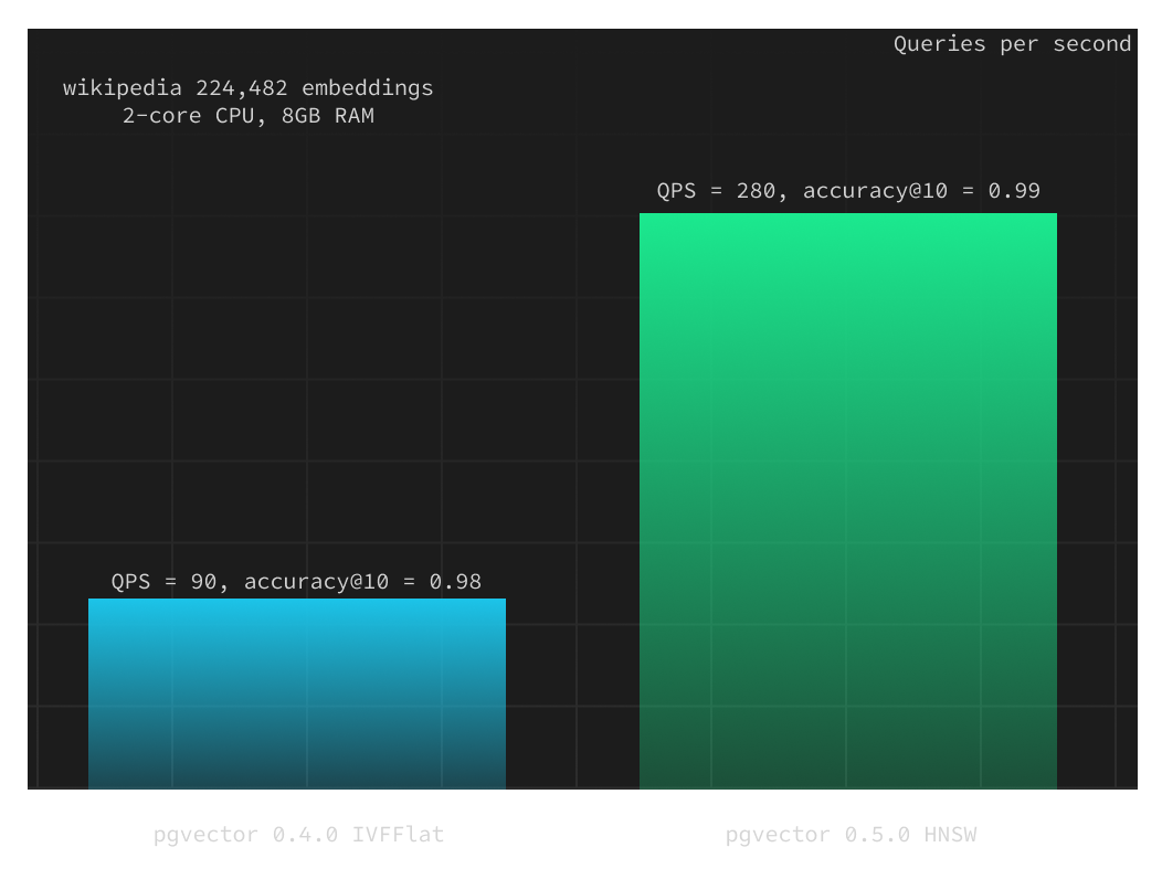
HNSW has 3 times better performance than IVFFlat and with better accuracy.
dbpedia-entities-openai-1M
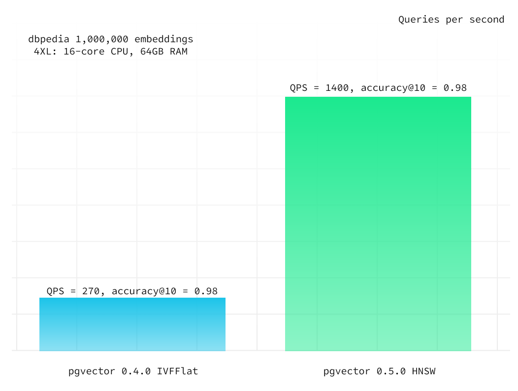
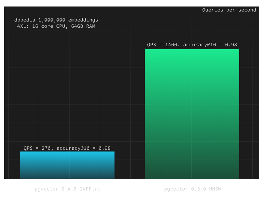
Next, we took the setup from our benchmarks with 1,000,000 vectors by OpenAI (1536 dimensions). If you want to find out more about pgvector 0.4.0 IVFFlat performance and our load testing methodology, check out pgvector 0.4.0 performance blogpost.
Here we used the Supabase project with a 2XL compute add-on (8-core CPU and 32GB RAM) and built the HNSW index with the same parameters:
m: 24ef_construction: 56
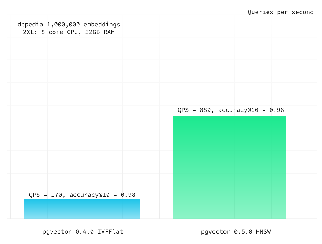
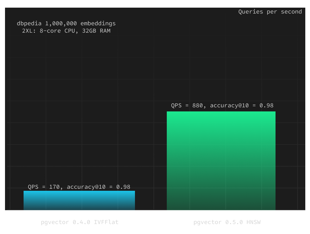
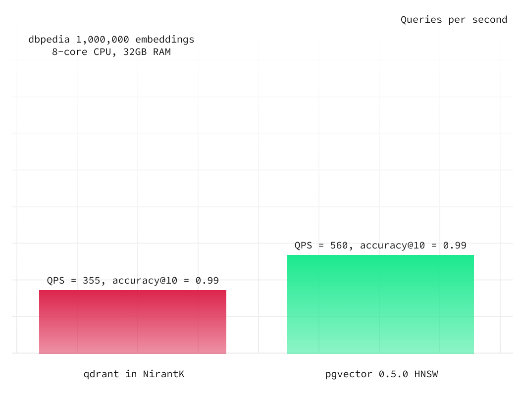
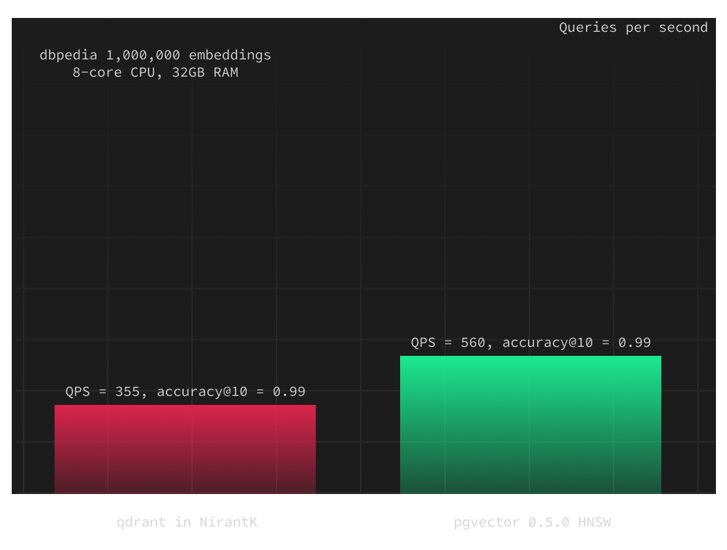
When we maintain fixed HNSW build parameters, we can adjust the select query parameter ef_search to balance query speed and accuracy. To achieve accuracy@10 of 0.98, we increased it from the default 40 to 100. For accuracy@10 of 0.99, we further raised it to 250. Remarkably, HNSW demonstrated over six times better performance while maintaining the same level of accuracy. With higher accuracy@10 of 0.99 HNSW even outperforms qdrant on equivalent compute resources.
Scaling the database
Performance scales predictably with the size of the database for the HNSW index, just as it does for the IVFFlat index. The difference in performance between IVFFlat and HNSW remains consistent after a compute upgrade.
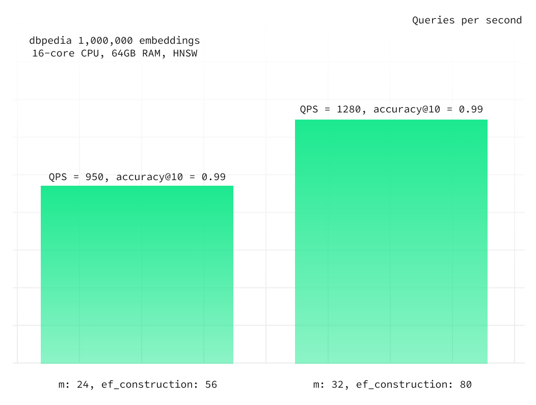
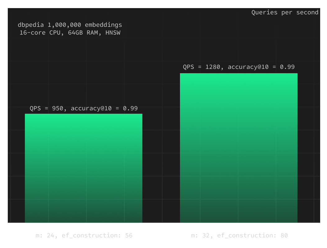
Switching to a 4XL compute add-on (with a 16-core CPU and 64GB of RAM) resulted in a 69% increase in QPS for an accuracy@10 of 0.99 compared to the 2XL instance.
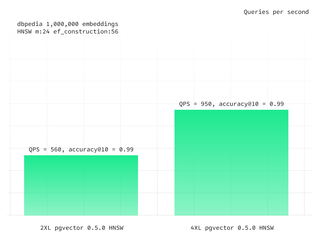
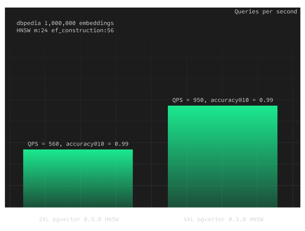
Furthermore, having 64GB of RAM is better suited for this dataset because Postgres uses approximately 30-35GB of RAM to achieve optimal performance. With a 4XL setup, you not only have the capacity to store 1,000,000 vectors but also the flexibility to accommodate additional data or increase the number of vectors as needed.
HNSW build parameters
We conducted a small experiment to assess the impact of HNSW index parameters on accuracy and QPS. In this experiment, we utilized the same 4XL instance as in the previous test but modified the building parameters:
m: 32ef_construction: 80
This adjustment enabled us to achieve the same level of accuracy@10 of 0.99 with an ef_search = 100 instead of the previous 250, resulting in a 35% increase in QPS.
Other HNSW features
In addition to the above query performance improvements, HNSW offers another advantage: you don't need to fully fill your table before building the index.
With IVFFlat indexes, the clusters (lists) are constructed based on the distribution of existing data in the table. This means that IVF indexes built on an empty table would produce completely suboptimal centers. This is why pgvector recommends building IVF indexes only once sufficient data exists in the table and rebuilding them any time the distribution of data changes significantly.
HNSW indexes use graphs which inherently are not affected by this limitation, so you are safe to create your HNSW index immediately after the table is created. As new data is added to the table, the index will be filled automatically and the index structure will remain optimal.
Improvements to IVF indexes
IVFFlat indexes also saw some improvements in v0.5.0. Index build times are now significantly faster for large datasets thanks to 2 new improvements:
- Parallelization during the assignment build step (assigning records to lists)
- Switching from double to float accuracy for select distance calculations which unlocks the fused multiply-add instruction on CPUs
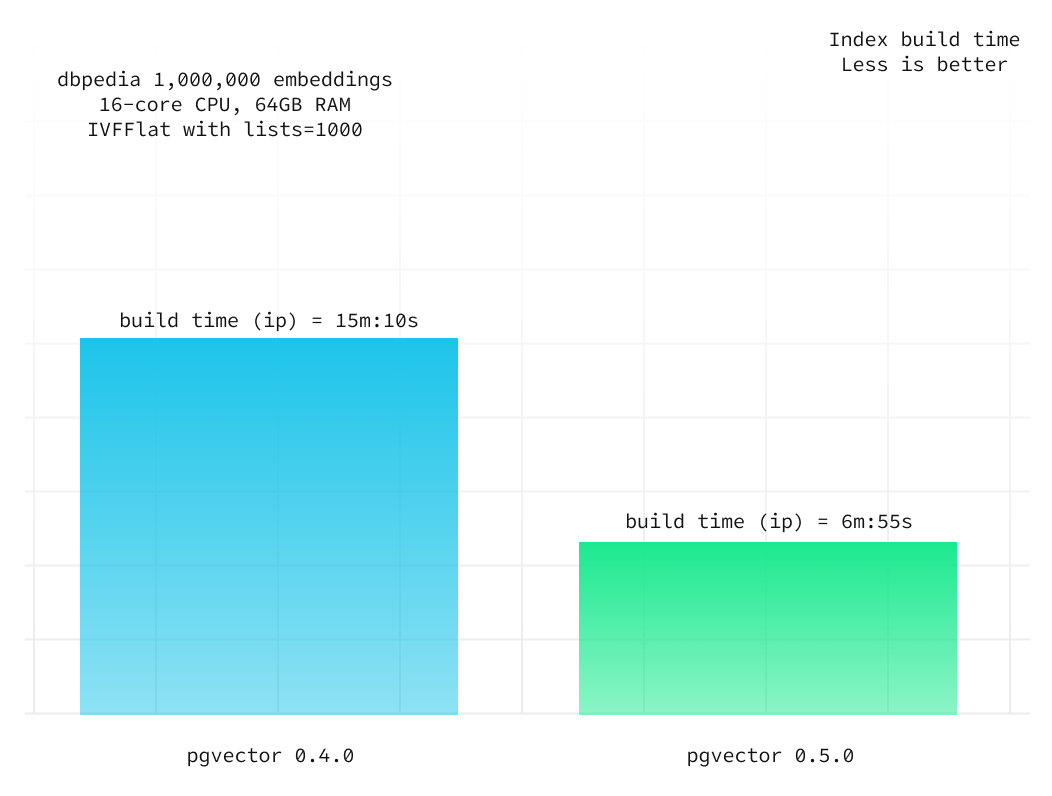
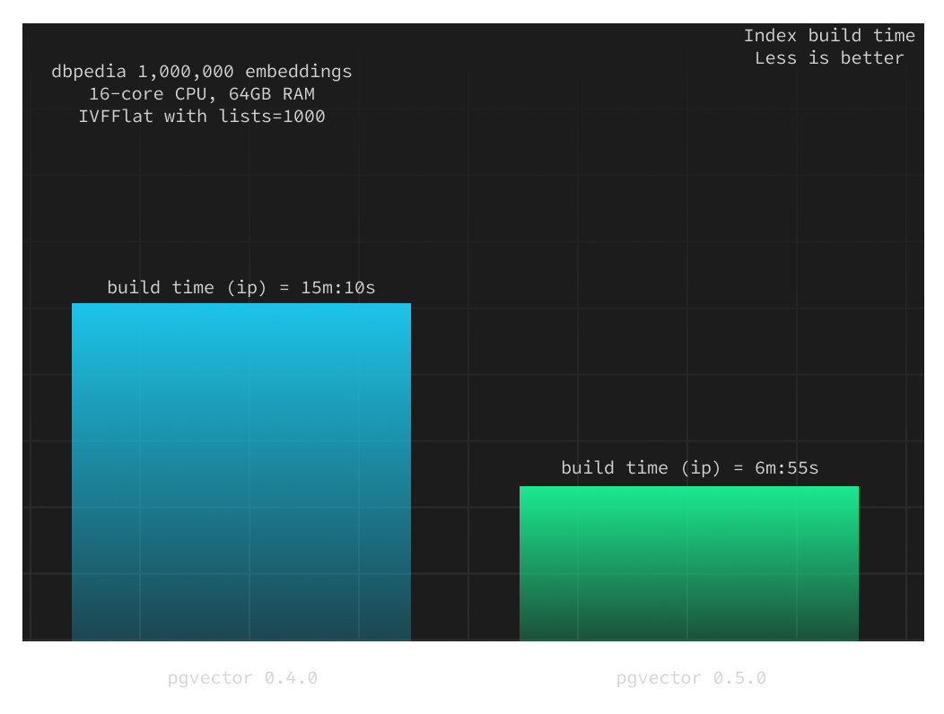
Below we compare the index build times between v0.4.0 and v0.5.0 for the inner product distance measure over 1,000,000 vectors on a Supabase project with 4XL compute add-on (with a 16-core CPU and 64GB of RAM).
lists = 1000
lists = 5000


The index build time has decreased by over 50%, and this ratio remains consistent when you adjust the index build parameters (specifically, the lists value).
When should you use HNSW vs IVF?
In most cases today, HNSW offers a more performant and robust index over IVFFlat. It's worth noting though that HNSW indexes will almost always be slower to build and use more memory than IVFFlat, so if your system is memory-constrained and you don't foresee the need to rebuild your index often, you may find IVFFlat to be more suitable. It's also worth noting that product quantization (compressing index entries for vectors) is expected for IVF in the next versions of pgvector which should significantly improve performance and lower resource requirements. Regardless of the type of index you use, we still recommend reducing the number of dimensions in your embeddings when possible.
Start using HNSW
All new Supabase databases will automatically ship with pgvector v0.5.0 which includes the new HNSW indexes. If you have an existing database, please reach out to support and we'll be more than happy to assist you with an upgrade.